Tutorial For Well-Sliced Metadynamics
Primary Reference:
See the paper: click here
Shalini Awasthi, Venkat Kapil and Nisanth N. Nair “ Sampling Free Energy Surfaces as Slices by Combining Umbrella Sampling and Metadynamics'' J. Comput. Chem. 37, 1413-1424 (2016).
Algorithm
Here, we briefly explain the algorithm for the well-sliced metadynamics (WS–MTD) approach. This technique requires no special implementation in a molecular dynamics.
code which can carry out well-tempered metadynamics (WT–MTD) simulation and umbrella sampling (US) runs simultaneously for different collective variables (CVs).
The reweighting procedure works as a post processing.
1. For the chosen range
of values of ![]() CVs,
place
CVs,
place ![]() restraining
umbrella potentials. For every umbrella, carry out a WT–MTD simulation sampling
the
restraining
umbrella potentials. For every umbrella, carry out a WT–MTD simulation sampling
the ![]() coordinates.
coordinates.
From these simulations, obtain the
time series of ![]() ,
,
![]() for
some regular intervals of MTD time
for
some regular intervals of MTD time ![]() .
.
2. Compute ![]() for
for
![]() .
.
3. Compute ![]() for
for
![]() .
.
4. Plot ![]() ,
and based on that choose a time range,
,
and based on that choose a time range, ![]() and
and
![]() ,
for which
,
for which ![]() ,
and a proper sampling of
,
and a proper sampling of ![]() has
been accomplished.
has
been accomplished.
5. For the time range, construct the MTD–unbiased distributions.
6. Using
WHAM, reweight the umbrella potential as well as combine the ![]() distribution
functions to get
distribution
functions to get ![]() .
.
Note that ![]() can
be the input for any standard WHAM programs, but by setting the bias along the
can
be the input for any standard WHAM programs, but by setting the bias along the ![]() coordinates
to zero.
coordinates
to zero.
7. Construct
the free energy surface ![]() .
.
Alanine-dipeptide
To study alanine–dipeptide, we use molecular dynamics using a Langevin thermostat at 300 K, with a time step 1.0 fs, using AMBER force–field. We employed the PLUMED–AMBER interface for carrying out WS–MTD runs (input files: plumed_input_file, amber_input_file, topology_file, coordinate_file).
In
WS–MTD simulations, ![]() coordinate is sampled using WT–MTD
and
coordinate is sampled using WT–MTD
and ![]() was
sampled using US. The choice of coordinates here is arbitrary. However, the US
coordinate is the one along which you are expecting a broad and/or unbound free
energy basin.
was
sampled using US. The choice of coordinates here is arbitrary. However, the US
coordinate is the one along which you are expecting a broad and/or unbound free
energy basin.
Here,
Gaussian potentials are updated at every 500 fs, and ![]() kcal
mol
kcal
mol![]() ,
,
![]() radians
and
radians
and ![]() K
are taken. Umbrella potentials are placed from
K
are taken. Umbrella potentials are placed from ![]() to
to
![]() at an interval of 0.2 radians with
at an interval of 0.2 radians with ![]() kcal
mol
kcal
mol![]() rad
rad![]() .
.
Details of the input files required for simulation can be found elsewhere.
Reweighting
Compile metadynamics unbiasing code.
$ gfortran mtd.f -o mtd.x
Prepare the input files (COLVAR, HILLS, run.sh).
If one is using PLUMED for running simulations output files can be directly used.
(Remove commented lines from COLVAR and HILLS file.)
COLVAR file should have following information
![]()
HILLS file should have the following information:
![]()
run.sh has following information:

Run command run.sh for processing files from different umbrella windows.
$ sh run.sh
Output file: Probability file (Pu.dat). Rename it as PROB_i, where “i” is the umbrella index.
These PROB files contain values for CV1, value for CV2, and probability of (CV1,CV2).
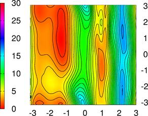
PROB files should be plotted to see the overlap between different umbrellas. If one finds insufficient overlap, then
more umbrellas can be simulated for intermediate values.
Collect all the PROB_i files in a folder PROB.
These PROB_i are the input for WHAM analysis.
Compile the WHAM code
$ mpif90 wham.F90 -o wham.x
Prepare WHAM input files (WHAMINPUT, input).
input file contain following information:

Temperature of physical system should be provided in Kelvin. Here, grid information should be same as used during MTD unbiasing.
WHAMINPUT file contains following information:
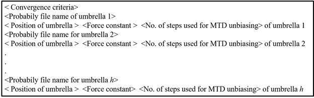
Run the executable (wham.x).
$ mpirun –np 8 wham.x (Running on 8 processors)
or
$ ./wham.x
Input file: PROB_i, WHAMINPUT, input
Output file: free_energy, which contains the free energies.
Free energies can be plotted using gnuplot using fes.gnp .