Workflow
Overview
Create a mol2 file of the molecule to parametrize.
Get CHARMM Additive parameters from CGenFF.
If polarizable Drude force field parameters are required, use CGENFF to Drude FF converter in FFParam. Double check its authenticity.
Test the performance of obtained CGenFF paramaters against target data obtained from QM calculations via:
Structural Similarity | * Visual comparison of optimized cartesian coordinates of QM and MM. | * Numerical comparison of optimized internal coordinates of QM and MM.
Electrostatic Parameters | * Comparison of water interaction energy of QM and MM to optimize partial atomic charges. | * Comparison of dipole moment of QM and MM for finding balance amongst partial atomic charges. | * Comparison of Molecular Polarizability of QM and MM for Alpha and Thole values in Drude FF.
Bonded Parameters | * Comparsion of Bond, Angle Dihedral Potential Energy Scan in QM and MM for conformational behaviour.
If the performance of some parameters are not satisfactory…
Change the associated paramater.
Rerun MM calculation.
Check performance of changed paramater against relevant QM target data.
If step 5 seems tedious, you may try Autofitting algorithms.
MCSA for charge, alpha, thole fitting.
LSFITPAR for bonded paramaters.
Note
Information on small molecule force field optimization for the additive force field based on CGenFF may be obtained from Kumar et al., 2019, Vanommeslaeghe et al., 2010 or Soteras Gutiérrez et al., 2016. For the polarizable Drude force field from Lemkul et al., 2016 or Lin and MacKerell, 2018. Additional information may be obtained from the MacKerell lab web page (http://mackerell.umaryland.edu/ff_dev.shtml).
Prerequisites for Parametrization
Tab: InitializeSystemSetup > ObtainCGENFFStr
Coordinate of the concerned molecule in .mol2 format is required. The additive force field Topology/Parameter file (.str file) for concerned molecule can be obtained from CGenFF .
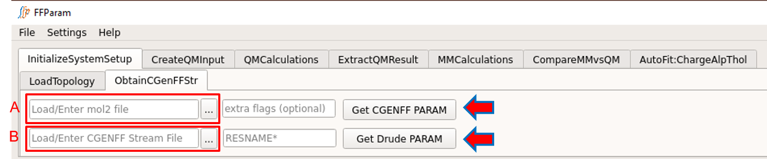
If CGenFF is locally installed and the path is linked in Settings, obtain resname.str file by supplying mol2 file in lineEditor A in ObtainCGenFFStr.
Extra flags available with CGenFF can be supplied in B.
Hit Get CGENFF PARAM.
Residue name in resname.str can be edited as required.
For the Drude force field:
First obtain additive toppar file i.e. resname.str and then convert to Drude atom types and parameters.
Supply an additive resname.str file in lineEditor C to obtain the resname_d.str file in drude format.
Resisude name must be mentioned in lineEditor D.
Hit Get Drude PARAM to get the resname_d.str file. Beware to check for the consistency of atom types and parameters in generated drude .str file.
Initialize the System (A required step)
Tab: InitializeSystemSetup > LoadTopology

Load the topology/parameter stream file (.str file) in lineEditor A.
The path of the .str file will be automatically loaded as the working directory in lineEditor B. User can change the working directory as needed, but this is not recommended.
Choose additive or drude in the dropdown menu C, depending on the type of .str file.
Enter residue name in lineEditor D. Correct residue name must be specified as information of this residue is read from the .str file. Notice that pushButton Load remains inactive till residue name is not entered/changed. This ensures that user provides all required information before proceeding.
- Hit pushButton Load. This performs a number of operations.* Activates all other tabs with atom, bond, angle and dihedral information (derived from .str file).* Based on type of force field, recommended level of theory and basis-set information is loaded in relevant tabs for creating QM Input files.* Other recommended parametrization rules such as scaling factor are loaded in the relevant tabs.* Activates pushButton F and G.* A restart file is created in the working directory containing the information provided in this tab. This restart file is automatically read when restarting FFParam-Gui from within the working directory.
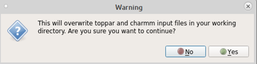
- Click on pushButton Fetch MM Prerequisites to transfer Charmm files from package repository to your working directory.* For additive force-field, it will transfer ffparam.inp, toppar.str, toppar_omm.str and the most recent toppar directory.* For drude force-field, it will transfer ffparam.inp, polar_efield.str, toppar_drude.str toppar_drude_omm.str and most recent toppar_drude directory.
If the system has previously been set up a warning will appear creation of the files is only required when the system is initially setup for parametrization.
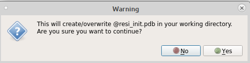
If a 3D structure of the molecule is needed Click on pushButton Generate Initial Coordinates. This creates initial coordinates that have the same atom names and order as in your .str file. Alternatively the desired coordinates may be accessed from mol2/pdb/crd format files. Important It is strongly recommended that the same atom order and names be in the .str and coordinate files as it greatly facilitates parameter optimization.
A warning may appear because the previous action will create/overwrite resname_init.pdb in your working directory.
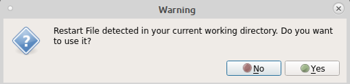
When ffparam-gui is launched subsequent times, a warning will appear asking whether or not to use the restart file created in the previous session. Once you accept, the information will be loaded. It is essential that pushButton Load be pressed before proceeding as this transfers the necessary information to the Gui as described above.
Inspect Structural Similarity
After initialization, the first step is to inspect how good or bad are the overall initial MM parameters. For this, the target data is optimized QM geometry and related properties like dipole moment.
Create QM Input for Geometry Optimization
Tab: CreateQMInput > Geometry Optimization
The geometry of the model compound should be intially be subjected to QM optimization at recommended level of theory and basis. In addition dipole moment and frequency calculations are performed.
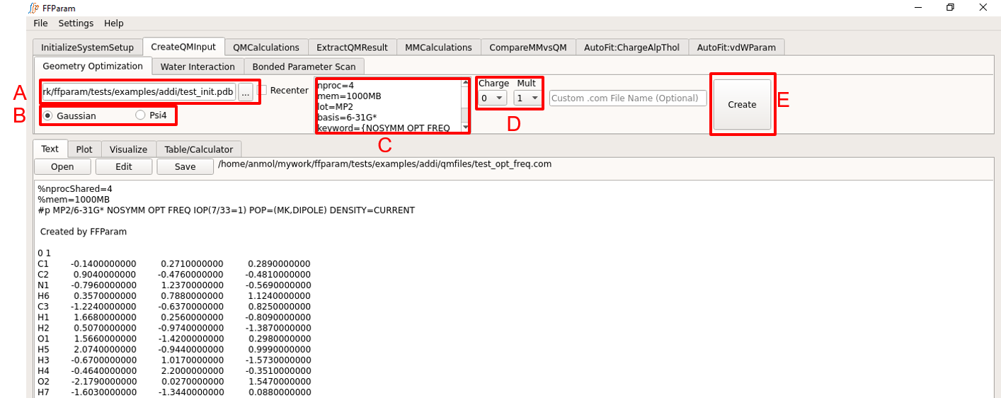
Load initial coordinate file (.mol2, .pdb, .crd formats accepted) in lineEditor A. You may instead choose to load resname_init.crd created using Generate Initial Coordinates.
Choose Gaussian or Psi4 format, B for the type of input file to be created.
Verify the default level of theory, basis-set and other keywords in textEditor C. You can change default values if you want.
Choose charge and multiplicity from dropdown menu D.
If custom name of input file is desired, provide the name with or without the path in lineEditor E.
Hit Create. A QM input file will be created in the qmfiles subdirectory under your working directory. The same file is displayed on textEditor G in the bottom section of FFParam-Gui. The symbols and the order of the atoms are the same as .str file provided during initialization.
Perform QM Calculations
Tab: QMCalculations
Run QM jobs locally
Gaussian: For running Gaussian job, path to Gaussian executable should be added in Settings Menu.
Psi4: For running Psi4 job, the executable does not need to be declared. Instead Psi4 should be installed in same enviornment or make sure Psi4 program library is added in PYTHONPATH.
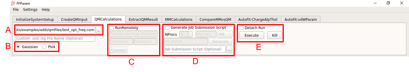
Load Input file in lineEditor A, which can be the input file created in the previous section. Supply only one input file, if you are running locally.
Select Gaussian or Psi4 B as per the format of the input file.
Hit Execute Button.
Consider detaching the job from the GUI as the QM optimization can be time consuming.
Run QM jobs remotely

First step before running a job on remote machine is to Connect Remote located in Settings. Provide IP address/alias name of remote machine, user name and password. Hit Connect to establish the connection. Connection Status is displayed in the bottom of the Remote Connection window.

More than one input files can be sent for QM calculation on remote machine (refer to lineEditor A).
If the connection was successfully established, the IP address/ alias name of the remote machine should appear in D.
Check E: RunRemotely to edit number of processors, per core memory, time limit, path where all the files will be placed on remote machine and path to Gaussian executable on remote machine. The default values for number of processors and memory are 4 and 1000 “MB”.

Hit G: Generate Script. This will create a number of job submission scripts equal to the number of input files provided in A and automatically place them in lineEditor H. The job submission script uses the template provided in Remote Connection window which can be modified except for the location of placeholders. Alternatively, you may supply a self-created job submission script.
Hit Execute to run the jobs on remote machine. The job-id’s on remote machine should appear in I, for which you may check the running status and get the output upon completion.

In the case of Psi4 jobs: Do not provide path of bin directory of remote machine containing psi4 executable. Rather, the path of Psi4 package on remote machine should be provided in lineEditor K. The QM jobs related to water interaction and potential energy scans in Psi4, contain instructions and the coordinates in different files. The instruction file should be supplied in lineEditor A while the coordinate files should be supplied in lineEditor J.
Alternatively, the input files created by CreateQMInput that are located in the qmfiles subdirectory may be transferred to a separate computational facility to perform the QM calculations. Once the calculations are finished, the output files should be transferred back to your workstation and placed in the qmfiles subdirectory.
Extract QM Results
Tab: ExtractQMResults
Extract the relevant information from qm output files (Gaussian -> .log / Psi4 -> .out). The QM geometry optimization output files contain the optimized geometry, internal coordinates, dipole moment and molecular polarizability if default keywords were used while creating QM input file.
Extract Optimized QM Geometry
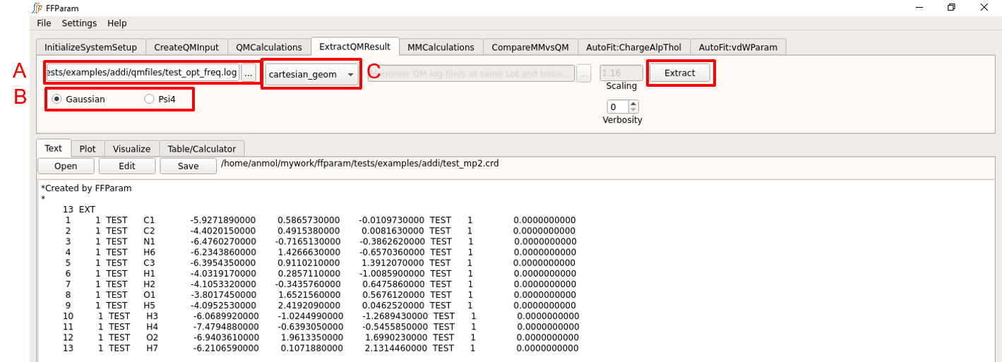
Load the QM output file in lineEditor A.
Choose if the output file is from Gaussian or Psi4 in B.
Choose cartesian_geometry from dropdown menu C to extract the geometry.
Increase verbosity D to get informed about background activities.
Hit Extract. The extracted geometry is saved as resname_mp2.crd file in the working directory. (mp2 in filename signifies level of theory.) The extracted coordinates are also shown in the TextEditor.
Extract Internal Coordinates
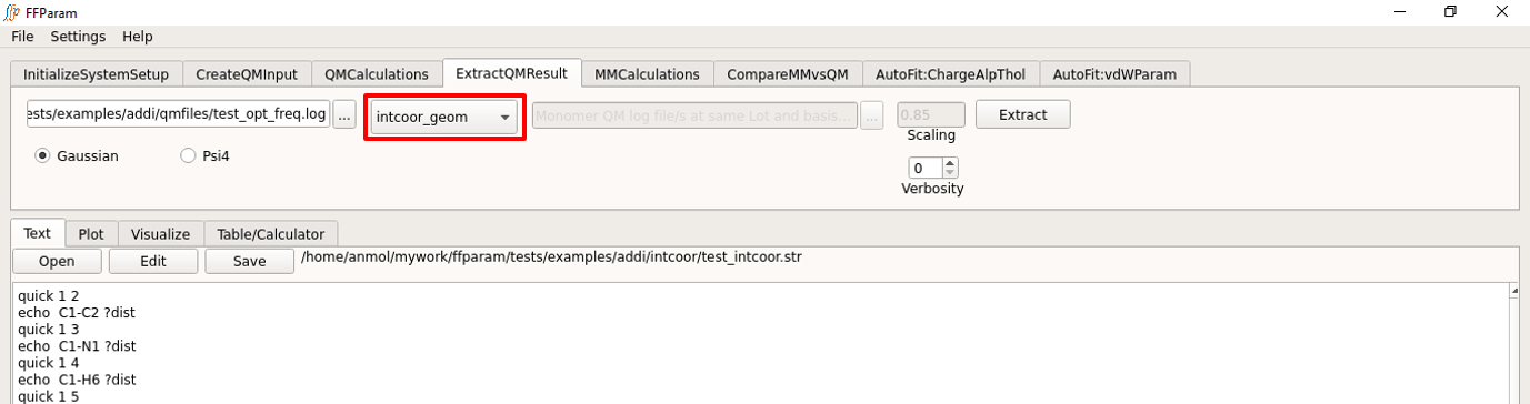
Load the QM output file in lineEditor A (This file is typically already loaded in the previous steps).
Choose if the output file is from Gaussian or Psi4 in B.
Choose internal_coordinates from dropdown menu C to extract the internal coordinates.
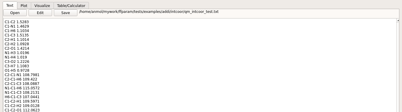
Hit Extract. The extracted internal coordinate is saved in qm_intcoor_resname.txt file placed in intcoor subdirectory.
In addition, step 4 creates the file “resname_intcoor.str” and places it in the intcoor subdirectory. This is required for internal coordinate evaluation in CHARMM.
Extract Dipole Moment and Polarizability
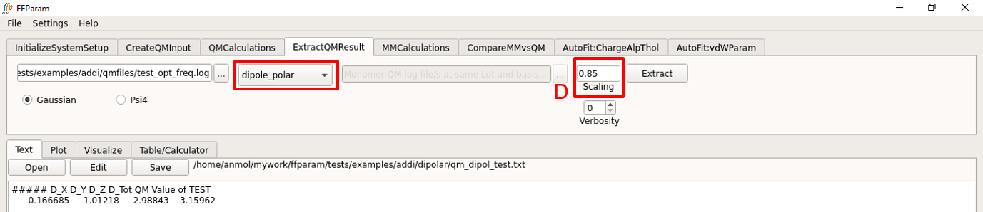
Load the QM output file in lineEditor A (This file is typically already loaded in the previous steps).
Choose if the output file is from Gaussian or Psi4 in B.
Choose dipole_polar from dropdown menu C to extract the dipole moment or polarizability.
Verify scaling factor in F.
Hit Extract. The extracted dipole/polarizability value is saved in qm_dipol_resname.txt placed in dipolar directory under working directory.
Note
The default keywords provided during CreateQM > Geometry Optimization does not contain POLAR keyword required for calculating QM molecular polarizability. In the case of Drude FF parametrization, a single point calculation on the optimized geometry should be performed at MP2/cc-pVQZ with POLAR keyword. Do not forget to remove OPT keyword. The output of this calculation should be used for getting target dipole and polarizability data for drude FF parametrization.
Perform MM Calculations
Tab: MMCalculations
CHARMM: For running CHARMM job, path to CHARMM executable should be added in Settings Menu.
OpenMM: For running OpenMM job, the executable does not need to be declared. Instead OpenMM should be installed in same enviornment or make sure OpenMM program library is added in PYTHONPATH.
Geometry Minimization in MM
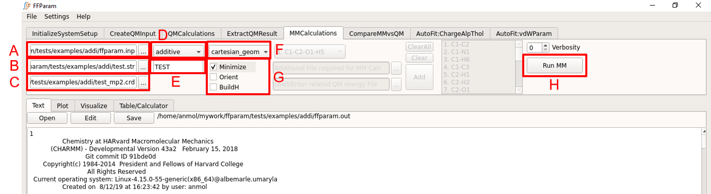
Load ffparam.inp in lineEditor A. This file is placed in the working directory by clicking Fetch MM Prerequisites button in the InitialSystemSetup.
Note
Prior to performing the MM calculation, toppar.str/toppar_drude.str files may be edited to avoid reading unnecessary topology and parameter files. For example, if the molecule is based solely on CGenFF atom types and parameters only the CGenFF toppar files along with the toppar_water_ions.str file need to be read via toppar.str.
Provide .str file containing topology and parameters in lineEditor B.
Provide coordinate file (recommeded: resname_mp2.crd containing the optimized QM coordinates) in lineEditor C.
Declare type of force-field (additive/drude) in dropdown menu D.
Enter resname in lineEditor E.
Choose cartesian_geometry from dropdown menu F.
Check Minimize option in G. Other options Orient and BuildH are optional and should not usually be checked.
Choose H: CHARMM or OpenMM to perform the calculation.
Note
ffparam.inp file is not used by OpenMM. Functionalities of OpenMM are limited to additive FF.
Hit Run MM to perform the calculation. While the calculation is running, Run MM button will remain inactive. Once the calculation is done, the output file “ffparam.out” will be displayed in the Text window and be available in the working directory.
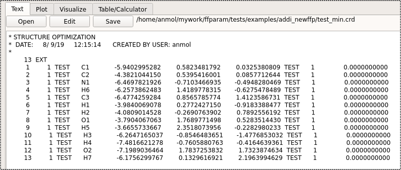
Additional files “resname_min.pdb” and resname_min.crd are generated in the working directory.
Internal Coordinates
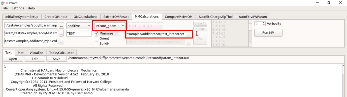
Steps 1, 2, 3, 4 and 5 above do not have to be repeated.
Choose internal_coordinates from the dropdown menu F.
Supply additional file required for MM Calculation of internal coordinates, i.e. “resname_intcoor.str” in intcoor subdirectory in lineEditor J.
Choose H: CHARMM or OpenMM to perform the calculation.
Hit Run MM to perform the calculation. Once the calculation is done, the output file “ffparam_intcoor.out” will be displayed in textEditor and written in the intcoor subdirectory.
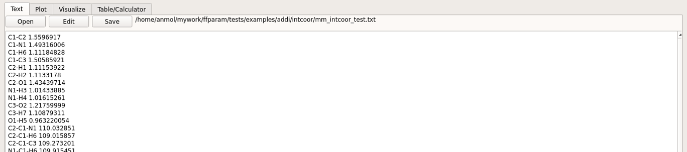
Internal coordinates are saved in mm_intcoor_resname.txt file placed in intcoor subdirectory.
Dipole Moment and Molecular Polarizability
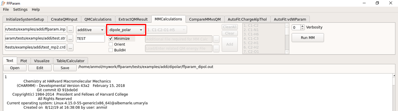
Steps 1, 2, 3, 4 and 5 above do not have to be repeated.
Choose dipole_polar from the dropdown menu F. In case of drude force-field, MM polarizability is also calculated.
Hit Run MM to perform the calculation. Once the calculation is done, the output file “ffparam_dipol.out” will be displayed in textEditor and written in the dipolar subdirectory..

All the components of dipole moment and molecular polarizabilities are saved in mm_dipol_resname.txt file placed in the dipolar subdirectory. Note that molecular polarizabilities are only present with Drude polarizable MM calculations.
Compare QM and MM Results
Geomteries
Tab: Visualize
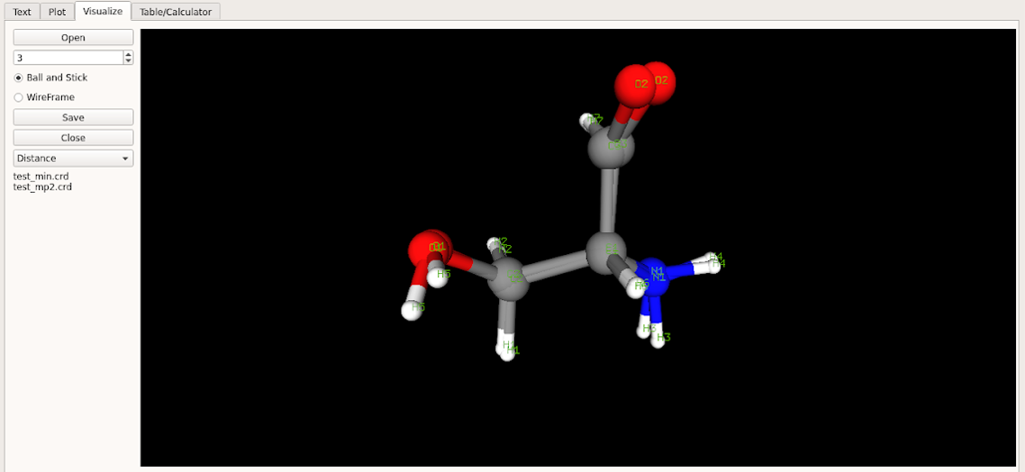
Before initiating the optimizaiton process compare the QM and MM minimized geometries based on the current parameters. Assuming that initial parameters obtained from CGENFF are reasonable the initial MM optimization should produce a geometry that is similar to the QM geometry. Care must be taken in the case of compounds with rotatable bonds to assure that the MM and QM conformations are in the same minima (same geometric isomers). This may be performed by visual inspection or by analysis of the difference in the internal dihedral coordinates (see below). For visual inpection load the MM and QM geometries saved in resname_min.crd and resname_mp2.crd; both files should be selected (cntrl mouse) and then opened simultaneously in the visualizer.
Internal coordinates
Tab: CompareMMvsQM
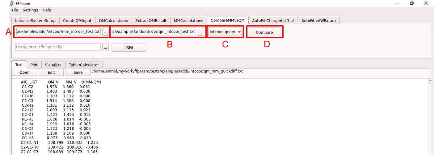
Choose internal_coordinates from dropdown menu A.
Load MM internal coordinates contained in mm_intcoor_resname.txt from the intcoor subdirectory in lineEditor B.
Load QM internal coordinates contained in qm_intcoor_resname.txt from the intcoor subdirectory in lineEditor C.
Hit Compare.
Dipole/Polarizability
Tab: CompareMMvsQM
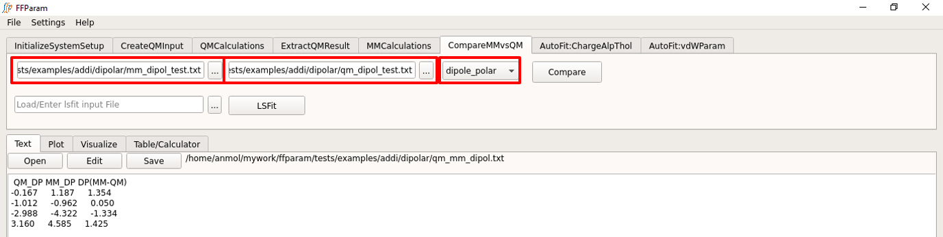
Choose dipole_polar from dropdown menu A.
Load MM dipole/polarizability contained in mm_dipol_resname.txt from the dipolar subdirectory in lineEditor B.
Load QM dipole/polarizability contained in qm_dipol_resname.txt from the dipolar subdirectory in lineEditor C.
Hit Compare.
Fit Electrostatic Parameters
Electrostatic parameters include charges in the additive force field while the Drude force field also includes alpha (atomic polarizabilities) and Thole scale factors. At the small molecule level these parameters are typically fit targeting interactions with water and dipole moments in the case of additive FF and with molecular polarizabilies in the case of the Drude FF. This step is typically performed using the QM optimized geometry, though the MM optimized geometry may be used if desired.
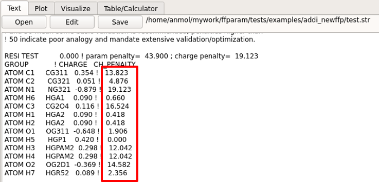
The electrostatic parameters do not have to be optimized for all the atoms. Atoms may be selected based on high penality values for the charges in .str file. If a subset of atoms are selected then water interactions only with those and adjacent atoms need to be used for generating target data. In general, water interactions should just be calculated for polar atoms.
Create QM Water Interaction Input Files
Tab: CreateQMInput > Water Interaction
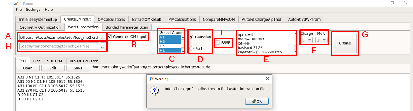
Load QM optimized geometry (.pdb or .crd or .log format) in lineEditor A.
Check B if you want to create QM input files.
Select atoms in C for which water interactions are to be calculated.
Note
If you do not check B and do not provide any resname.da file in lineEditor I, a resname.da file will be created for the selected atoms and will be placed in charges subdirectory. If you know the format of .da file and provide one in lineEditor I, it will supersede the choice of selected atoms in C and will rather be used to create the QM input files. resname.da file contains the selected atoms, their neighbors and some values required to place the water molecules around the model compound. The same resname.da file is used during calculation of MM water interactions.
Choose between Gaussian and Psi4 formats in D for the type of input file to be created. Check FAQ for recommended level of theory and basis-set.
Check E if you want to include BSSE correction.
Verify the default level of theory, basis-set and other keywords in F. The default values may be changed by the user.
Choose charge and multiplicity from dropdown menu G.
Hit H: Create. Since multiple water interaction files are usually generated, the textEditor displays the resname.da.
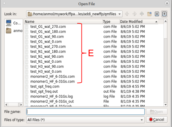
Check the water interaction QM input files in the qmfiles subdirectory. resname_atom_wat_LP.com or resname_atom_wat_LN.com files contain parent geometry along with geometry of water placed in a particular orientation. LP denotes that water molecules are placed in the direction of lone pair of the selected acceptor atom, while LN denotes linear orientation of water molecules. 1 and 2 denote two different orientations of 2nd hydrogen atom in water molecule. Notice that “monomer1_lot_basis.com” and “monomer2_lot_basis.com” files are also created. This is used for obtaining monomer energies at the same level of theory and basis-set. In the case of Psi4, each water interaction input file is split into two different files i.e. .py and _xyz.py containing instructions and coordinates, respectively.
For each non-hydrogen atom selected for water interaction calculation, you might see four different QM input files (containing four different orientation of water molecules against parent molecule). You should choose to do QM calculation on only those files, which show (visual inspection is required for steric clash) maximum interaction with the concerned atom and minimum interaction with other atoms in the parent molecule. The idea is to obtain interaction energy with maximum contribution from the concerned atom and least interaction with other atoms. The visual inspection can be done by loading the .com or _xyz.py files in Visualize tab of FFParam.

Above figure shows 4 different orientation of water molecule created for checking the interaction with O2 atom in the molecule. Here O2-LP1 orientation may be discarded because one of the hydrogen atoms in the parent molecule is in close proximity with water molecule. The entry regarding O2-LP1 (A2 O2 0 A B) in resname.da should also be removed because resname.da is used during MM calculation to obtain corresponding interaction energies.
Perform QM Calculations on the QM water interaction files. These may be performed using the QM Calculations tab as described above or on a separate computational facility. The QM output files should ultimately be placed in the qmfiles subdirectory.

Above figure describes the notation used in creating dafile.
Extract QM Water Interaction Energies
Tab: ExtractQMResults
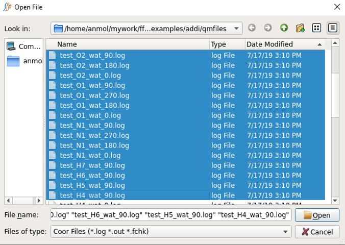
Select all the desired resname_da_wat.log or .out files at once in lineEditor A, except the monomer files.
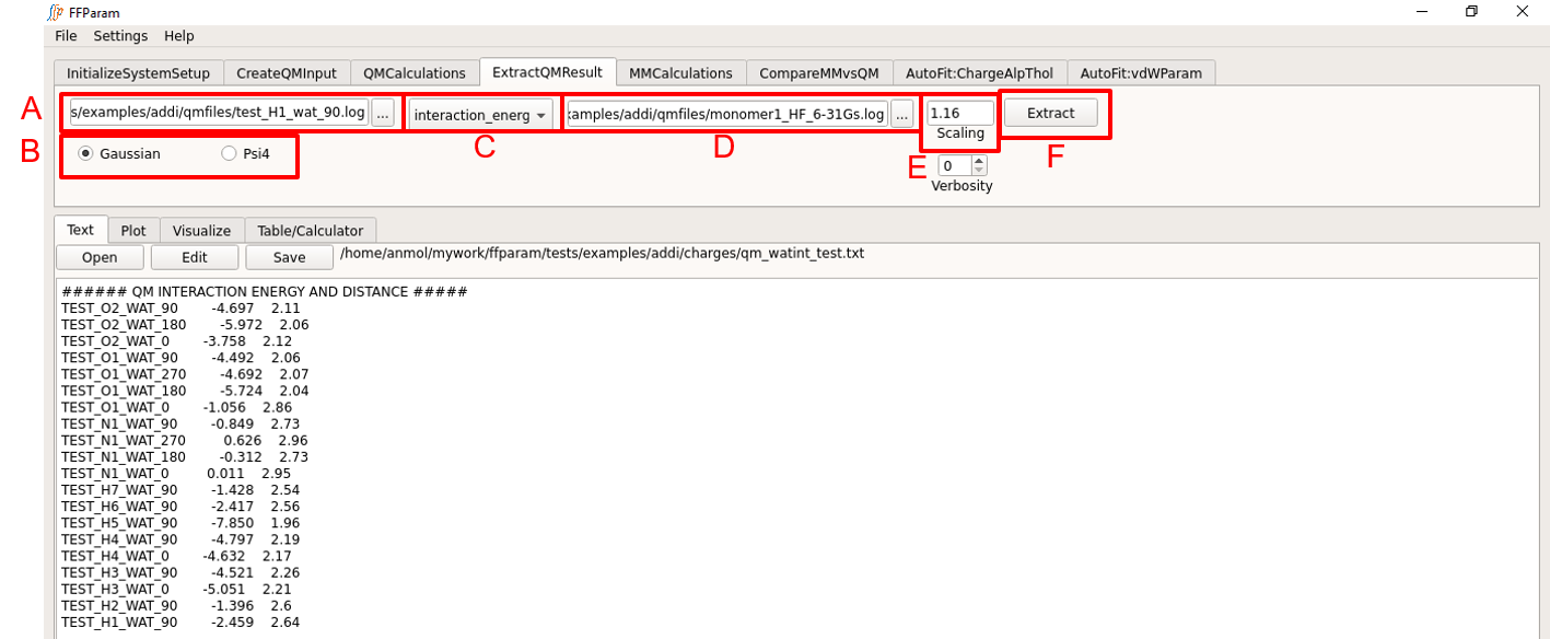
Choose if the output files are from Gaussian or Psi4 in B.
Choose interaction_energy in dropdown menu C.
Provide both monomer_lot_basis.log or .out files in lineEditor D. Select both files simultaneously. This is required for obtaining the monomer energies.
Verify the scaling factor in E. 1.16 for neutral molecules, 1.0 for charged or sulfur containing molecules. 1.0 for the Drude FF.
Hit Extract. A file qm_watint_resname.txt containing designators, QM minimum interaction energies and distances will be created for the selected QM output files. This file is placed in the charges subdirectory.
Perform MM Interaction Energy Calculation
Tab: MMCalculations
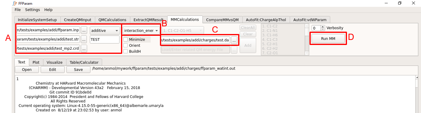
Typically steps 1,2,3,4,5 related to block A are same as before. Check Perform MM Calculations. Be careful about the version of resname.str being uploaded if changes in the parameters have been made.
Choose interaction_energy from dropdown menu B.
Provide resname.da file created above in lineEditor C. The .da file is converted into resname_watint.str file before running the MM calculation. So if this step was run previously, “resname_watint.str” file may be supplied in lineEditor C.
Hit Run MM to perform the calculation using CHARMM or OpenMM. Once the calculation is done, the output, “ffparam_watint.out” will be displayed in textEditor and located in the charges subdirectory.
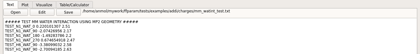
A mm_watint_resname.txt file is also created in the charges subdirectory analogous to the “qm_watint_resname.txt” file. These files are used for comparing the QM and MM results.
Compare MM and QM Interaction Energies
Tab: CompareMMvsQM
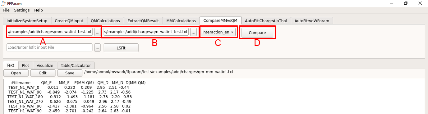
Choose interaction_energy in dropdown menu A.
Load mm_watint_resname.txt in the charges subdirectory in lineEditor B.
Load qm_watint_resname.txt in the charges subdirectory in lineEditor C.
Hit Compare. The results are shown in the Text window and a file containing comparision of energies and distances is created in the charges subdirectory. Names that are common in the first column of both files are used for evaluation.
Depending on the difference, you may decide whether or not partial charges require further optimization. It is advised to have difference between QM and MM interaction energy below 0.5 kcal/mol.
Manual Fitting of Charges
Table/Calculator
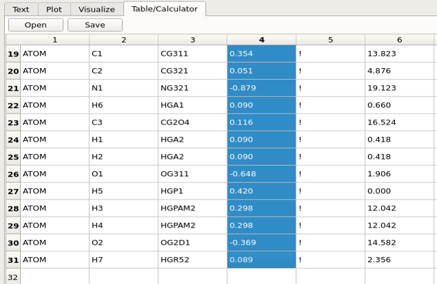
To fit the charges (or other electrostatic parameters) manually, the charges in the .str need to be modified. This is best performed by opening the .str file in the Table/Calculator window. This allows for the charges to be edited and, importantly the functionality of the Table/Calculator window allows columns or rows of numbers to be selected and the sum returned. This is required as the sum of the charges needs to be an integer that is equal to total charge. To perform this operation select all the charges and then clck anywhere within the selection, which will return the total charge on in the terminal from where FFParam-Gui was launched. Once the new charges are assigned repeat the MM Calculation of the interaction energies followed by Compare MM and QM Interaction Energies to determine the extent of the improvement with respect to the interactions with water and dipole moment.
AutoFitting of charges
Tab: AutoFit:ChargeAlpThol
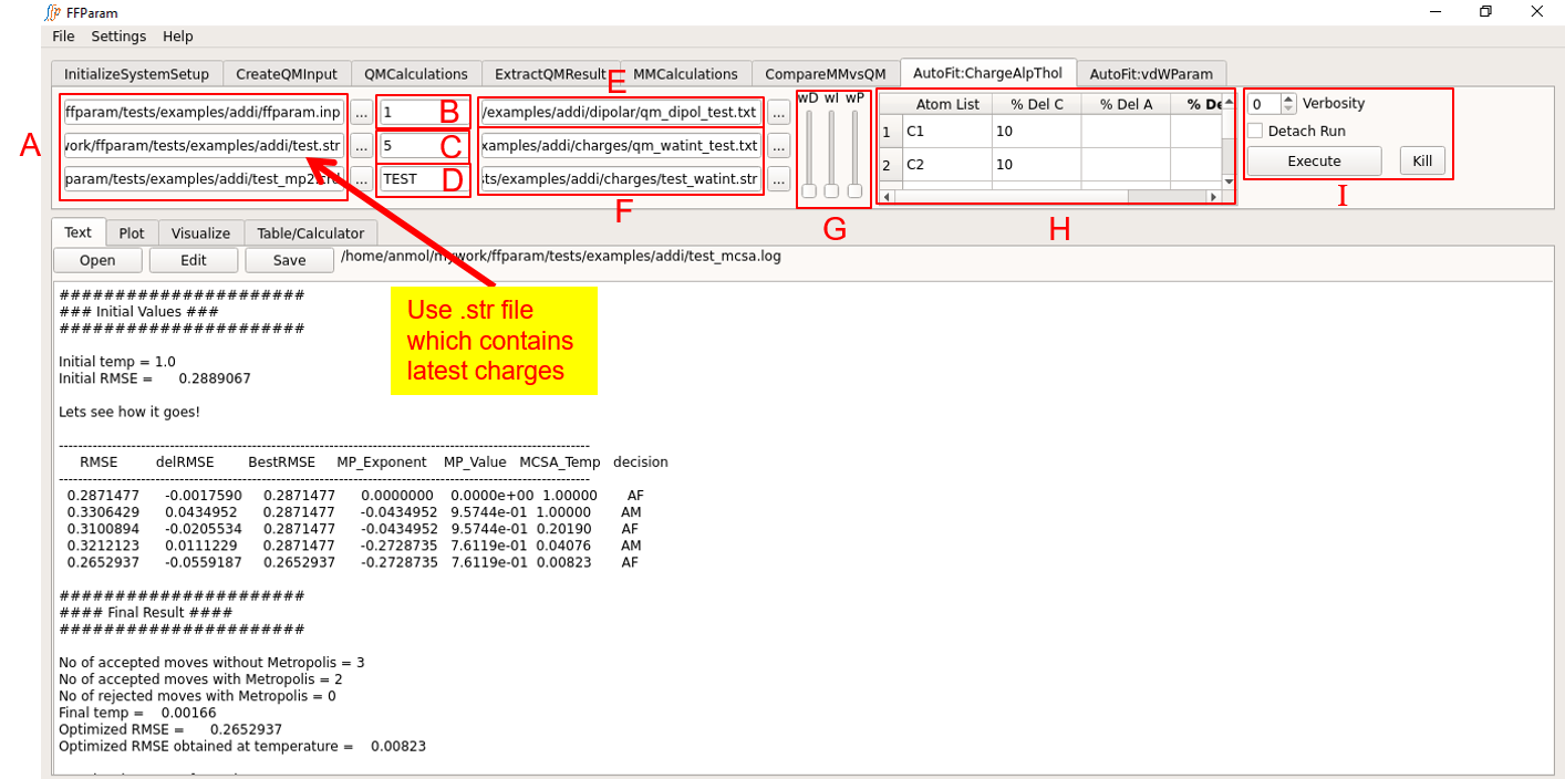
The block A contains ffparam.inp, resname.str and resname_mp2.crd as used during MM Calculation. Be careful about the version of resname.str you are uploading if changes in the parameters have been made.
Enter MCSA temparature in lineEditor B. Recommended value is 1.
Enter desired number of MCSA steps in lineEditor C. Recommended value is > 500.
Enter resname in lineEditor D.
Load qm_dipol_resname.txt file in lineEditor E. (Optional)
Load the qm_watint_resname.txt file and resname.da / resname_watint.str files from the charges subdirectory (created during MM interaction energy calculation) in F.
Note
Either one or both of the dipoles and water interactions (step 5 and 6) may be supplied as target data.
If both types of target data are given, assign weights using the slide bars in G. All slide bars at the bottom indicates equal weighting.
Default percentage change allowed for each partial charge parameter can be seend in Table H. This can control the extent of variation occurring on each atom and allows fixing the parameters on atoms by setting the percent change to 0. Note that charges on hydrogen atoms are fixed by default in CGenFF or DGenFF. The default values may be changed as per requirement.
Choose between CHARMM and OpenMM in I.
Hit Execute. The result is displayed in the TextEditor. A new stream file “resname_mcsa_bstrms.str” containing the fitted charge parameters along with the bonded parameters as present in the original resname.str is created in the working directory. A renamed version of this file may be used for subsequent parameter optimization.
Note
Do not run any other job through FFParam-Gui while MCSA is running.
AutoFitting of Alpha and Thole Parameters
Tab: AutoFit:ChargeAlpThol

Autofitting Alpha and Thole parameters is similar to the charge fitting. It is usually performed after the charges are optimized. For this fitting, qm_dipol_resname.txt should contain both dipole and molecular polarizability data. Typically the qm_watint_resname.txt target data is not be provided while performing alpha and thole fitting as the model is designed to reproduce gas phase dipole moments and molecular polarizabilities. Similar to the partial charges, the default percentage changes in alpha and thole parameters may be adjusted in table H before running MCSA.
Note
In practice it may be easiest to initially optimize the charges, alphas and Tholes targeting just the QM dipoles and molecular polarizabilities. The resulting electrostatic model may then be used to calculate the interactions with water for comparison with the corresponding QM data. Decisions may than be made concerning the need for additional electrostaic parameter optimization and/or the need for pair-specfic LJ (NBFIX) for NBTHOLE terms to improve specific interactions with water.
Fit Bonded Parameters
Bonded parameters include bond, angle and dihedral parameters. Improper and Urey-Bradley parameters may also be adjusted but only manually. This step is typically performed after charge fitting with the charges then reevaluated if the geometry of the model compound changes significantly.
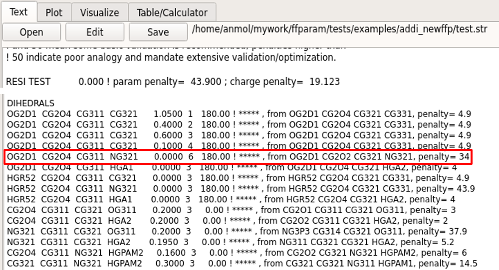
Bonded parameters for optimization may be selected based on high penality values in the .str file. Parameters related to those bonds, angles and dihedrals which show large differences between internal coordinates of QM and MM optimized structures can also be selected for optimization. Dihedral parameters involving aliphatic hydrogens atoms are typically NOT optimized. In general, parameters already available in CGenFF are not subjected to further optimization to maintain the integrity of the force field. However, the user may override this rule as their discretion.
Create QM Bond/Angle/Dihedral PES Input Files
Tab: CreateQMInput
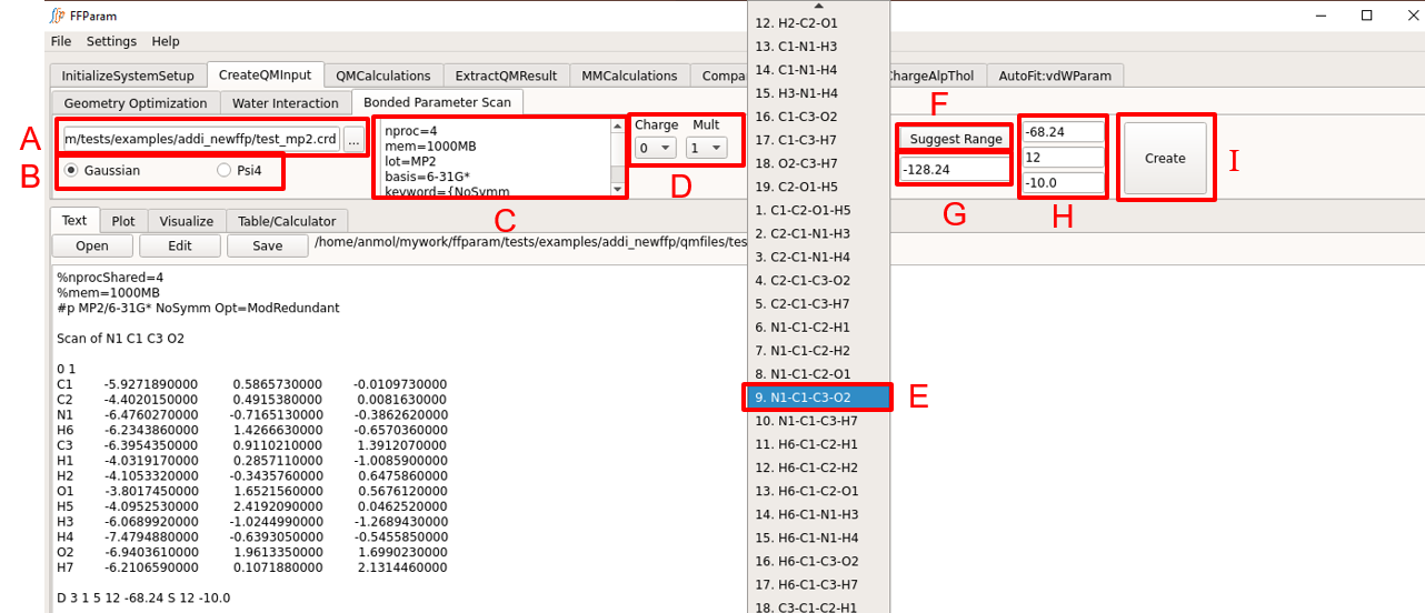
Load QM optimized geometry (.pdb or .crd or .log format) in lineEditor A.
Choose between Gaussian and Psi4 formats in B for the type of input file to be created.
Verify the default level of theory, basis-set and other keywords in textEditor C. Default values may be modified if desired.
Choose charge and multiplicity from dropdown menu D.
Choose internal coordinate for the PES from dropdown menu E. The tool-tip displays the atom type of the atoms in internal coordinates.
Click F: Suggest Range for getting initial value of choosen internal coordinate in lineEditor G. Starting value, number of steps and step size is popped in H. It can be changed as per requirement.
Hit I: Create. The created QM PES input file is displayed in textEditor.
Create individual QM input files for the PES scans of all selected internal coordinates. Perform QM Calculations and place the output files in the qmfiles subdirectory.
Extract Bond/Angle/Dihedral PES Result
Tab: ExtractQMResult
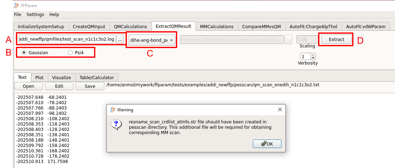
Select one QM scan output file in lineEditor A.
Choose if the output file is from Gaussian or Psi4 in B.
Choose dihe-ang-bond_pes in dropdown menu C.
Hit Extract. A file qm_scan_enetyp_atmnames.txt containing energies and bond/angle/dihedral values will be created and placed in pesscan subdirectory.
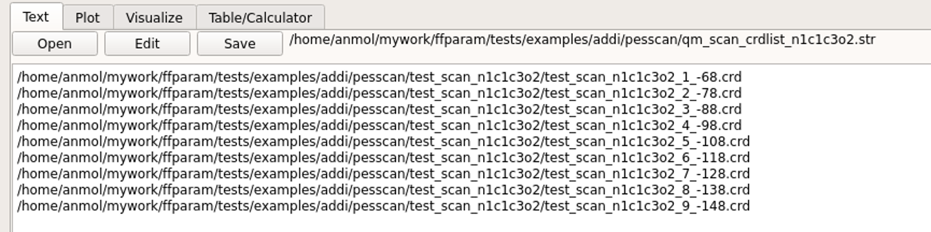
This also extracts optimized geometries of every scan step and places them in a subdirectory under the pesscan directory. An additional file qm_scan_crdlist_atminfo.str is created which contains the full path to extracted geometries. This information is used during corresponding MM scan.
Perform MM Bond/Angle/Dihedral PES
Tab: MMCalculations
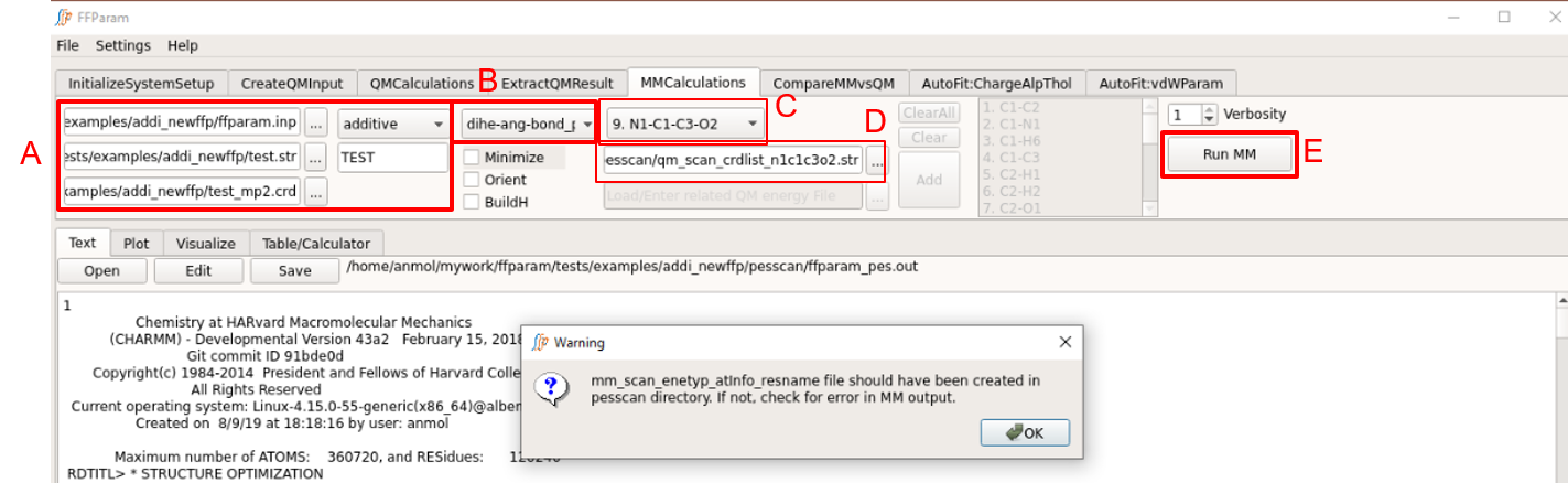
Treat A as performed above. Be careful about the version of resname.str being uploaded if changes in the parameters have been made.
Choose dihe-ang-bond_pes from dropdown menu B.
Choose a internal coordinate for performing MM scan from dropdown menu C.
Provide corresponding qm_scan_crdlist_atminfo.str file in lineEditor D which is created after extracting QM PES output file as described above.
Hit Run MM to perform the calculation. Once the calculation is done, the output, “ffparam_pesscan.out” will be displayed in textEditor and placed in the parent directory.
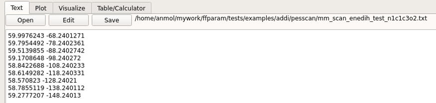
An additional file mm_scan_enetyp_atmnames.txt is created analogous to the qm_scan_enetyp_atmnames.txt file allowing for direct comparison of the MM and QM results.
Compare MM & QM PES
Tab: CompareMMvsQM
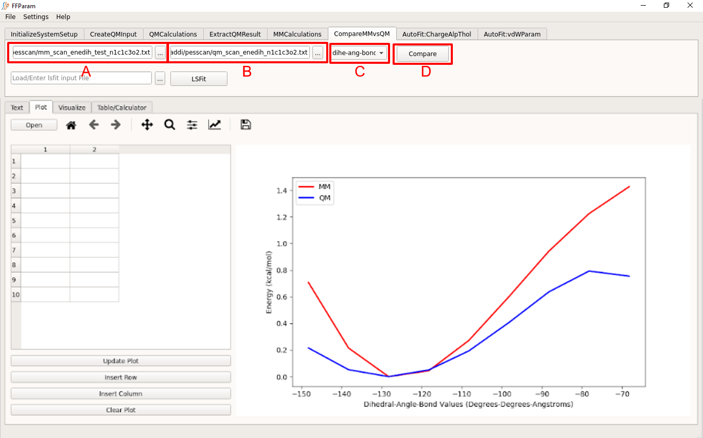
Load mm_scan_enetyp_atmnames.txt in lineEditor A.
Load qm_scan_enetyp_atmnames.txt in lineEditor B.
Choose dihe-ang-bond_pes in dropdown menu C.
Hit Compare. A comparison graph will be plotted in Plot.
Manual fitting of bonded parameters
Manual parameter optimization is often sufficent if only a couple of bond, angle or dihedral parameters require optimization. If there are more than this, automated optimization targeting QM PES is appropriate.
Bonded parameter optimization may involve optimization of: 1. The equilibrium bond and angle value. 2. Force constants can then be optimized to reproduce potential energy scans (PES) about the selected bonds, angles and dihedrals. 3. The diheral phases and multiplicity.
Optimization of bond and angle parameters does not always require corresponding QM PES data. If the difference between QM and MM bond and angle values is apparently large, the corresponding bond and angle parameter in .str file can be changed to minimize the difference. Value of bond and angle in QM optimized geometry serve as good guess for equilibrium bond and angle value in MM. After every change in the parameters, rerun MM minimization as in Perform MM Calculations and use Compare QM and MM Results to compare the optimized MM geometries with modified parameters against QM geometry.
An important issue to consider is that the equilibrium value of the angle parameters about planar (sp2) atoms should sum to 360 (acyclic atom), 540 (5-membered ring) or 720 (6-membered ring) for planar systems. To facilitate this the Table/Calculator capabilities may be used to sum the equilibrium parameters. Finally, it may not be feasible to exactly obtain 360, 540 or 720 due to certian parameters being fixed, but getting close to these values is suggested.
If QM PES data is available, these parameters should be changed such that MM PES matches well with QM PES atleast upto the value of 10 kcal/mol. This applies to dihedral fitting as well.
With dihedrals, there may be multiple multiplicities (n; 1, 2, 3, 4, 5 and 6) each with individual force constants and phases. It is desirable to minimize the number of multiplicities used for each dihedral as the individual terms can start to cancel each other (parameter correlation). Accordingly, testing the use of only one or two terms prior to going for more terms is strongly suggested.
Autofitting of Bonded Parameters
As described above if the QM and MM scans are similar it may be preferable and indeed time saving to manually optimize the associated parameters as this avoids setting up and performing multiple least-squares fitting runs. For automatic fitting of bonded parameters, download and install LSFITPAR. Provide executable path in Settings Menu. Using lsfitpar program requires preparation of the MM data files for the fit to be performed. FFParam-Gui may be used for this purpose as follows.
File Preparation for lsfitpar
Tab: MMCalculations
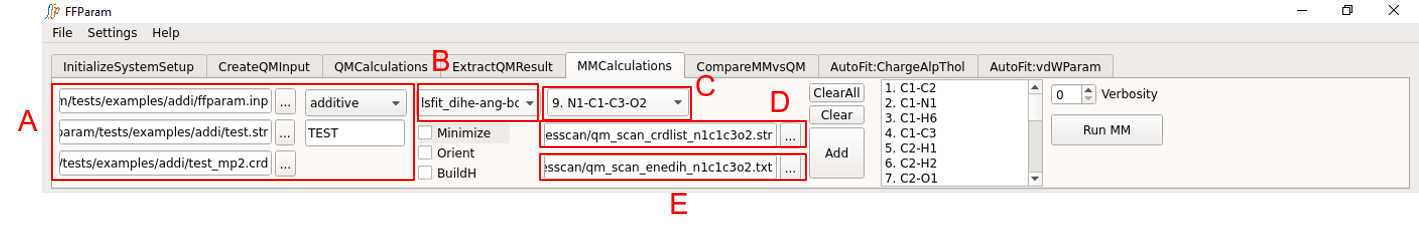
Step 1,2,3,4, and 5 related to block A are same as other MM calculations. Be careful about the version of resname.str being uploaded if changes in the parameters have been made.
Choose lsfit_dihe-ang-bond from dropdown menu B.
Choose a internal coordinate for fitting from dropdown menu C.
Provide corresponding qm_scan_crdlist_atminfo.str file in lineEditor D.
Provide corresponding qm_scan_enetyp_atmnames.txt file in lineEditor E.
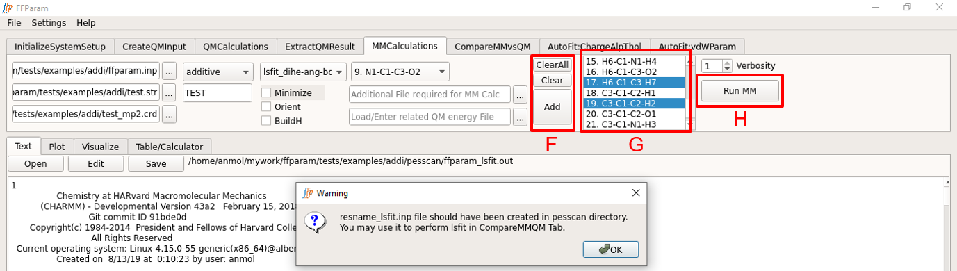
Click Add to add the files in D and E to a list. This action clears the field D and E. If you want to fit more than one bonded parameter, choose another dihedral, provide corresponding crdlist.str and energy.txt file and click add to append to the list. In case of a mistake, use clear or clear all buttons.
Choose other internal coordinates in I for measurement (usually bond and angle). This is optional but it enriches the matrix used by lsfitpar.
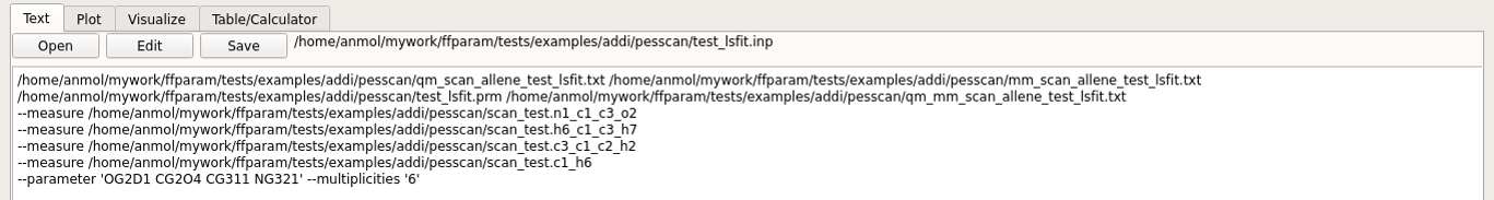
Hit Run MM to perform the calculation. Once the calculation is done, the output, “ffparam_lsfit.out” will be displayed in textEditor. This action creates several files in pesscan directory which are required by lsfitpar.
A input file resname_lsfit.inp for lsfitpar should be created in pesscan directory.
Execute lsfitpar
Tab: CompareMMvsQM
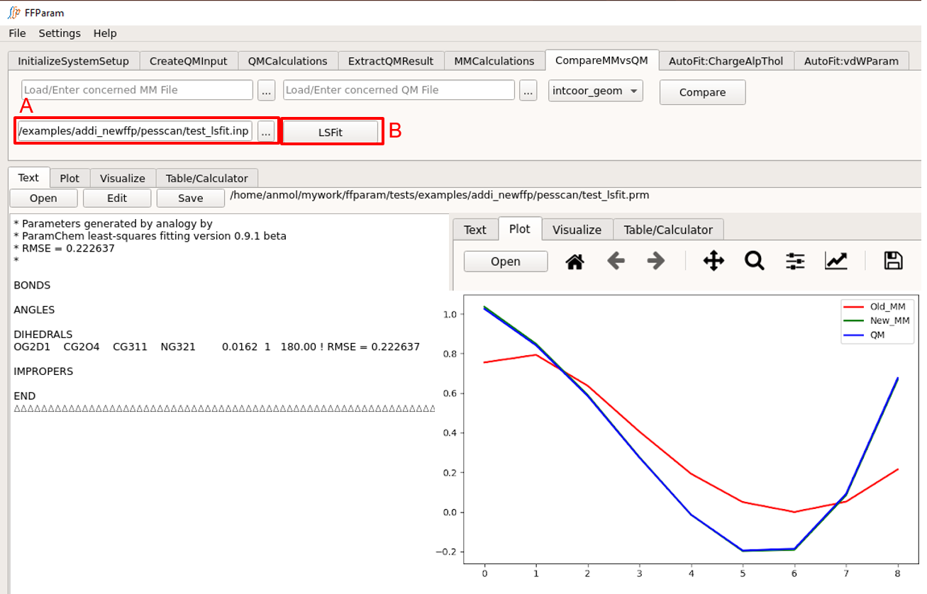
Load resname_lsfit.inp file in lineEditor A.
Hit LSFit. It produces both text and graph output. TextEditor and Plot is updated with the result of lsfitpar.
Following completion of the LSFit program check the ouptput .str file to determine if the optimized parameters are reasonable. Then use the new .str file to calculate the MM PES using Perform MM Bond/Angle/Dihedral PES and Compare MM & QM PES to verify that the optimized parameters reproduce the LSFit PES in the context of the full energy function in CHARMM or OpenMM.
References
Kumar, A., Yoluk, O., and MacKerell, A.D., Jr. “FFParam: Standalone Package for CHARMM Additive and Drude Polarizable Force Field Parametrization of Small Molecules,” Journal of Computational Chemistry, 2019, DOI https://doi.org/10.1002/jcc.26138
Guvench, O. and MacKerell, A.D., Jr., “Automated conformational energy fitting for force-field development,” Journal of Molecular Modeling, 14, 667-679, 2008, DOI 10.1007/s00894-008-0305-0, PMC2864003
Lemkul, J.A., Huang, J., Roux, B., and MacKerell, A.D., Jr. “An Empirical Polarizable Force Field Based on the Classical Drude Oscillator Model: Development History and Recent Applications,” Chemical Reviews, 116: 4983–5013, 2016, 10.1021/acs.chemrev.5b00505, PMC4865892
Lin, F.-Y. and MacKerell, A.D., Jr., “Polarizable Empirical Force Field for Halogen-containing Compounds Based on the Classical Drude Oscillator,” Journal of Chemical Theory and Computation, 14: 1083–1098, 2018, 10.1021/acs.jctc.7b01086, PMC5811359
Soteras Gutiérrez, I., Lin, F.-Y.,* Vanommeslaeghe, K.,Lemkul, J.A., Armacost, K.A., Brooks, Cl., III, and MacKerell, A.D., Jr., “Parametrization of Halogen Bonds in the CHARMM General Force Field: Improved treatment of ligand-protein interactions,” Bioorganic & Medicinal Chemistry, 24: 4812-4825, 2016, 10.1016/j.bmc.2016.06.034, PMC5053860
Vanommeslaeghe, K., Hatcher, E., Acharya, C., Kundu, S. Zhong, S., Shim, J., E. Darian, E., Guvench, O., Lopes, P., Vorobyov, I., MacKerell, A.D., Jr., “CHARMM General Force Field (CGenFF): A force field for drug-like molecules compatible with the CHARMM all-atom additive biological force fields.” Journal of Computational Chemistry, 31: 671-90, 2010, 10.1002/jcc.21367, PMC2888302
Vanommeslaeghe, K., Yang, M., and MacKerell, A.D., Jr., “Robustness in the fitting of Molecular Mechanics parameters,” Journal of Computational Chemistry, 36: 1083-1101, 2015, 10.1002/jcc.23903, PMC4412823